Inverse probability or odds weighting-based transportability analysis
Core Clinical Sciences
transportIP.Rmd#>
#> Attaching package: 'TransportHealth'
#> The following object is masked from 'package:base':
#>
#> truncIntroduction
In this vignette, we demonstrate how to use
TransportHealth for weighting-based transportability
analysis for instances where mergeable individual participant-level data
(IPD) are available in both the original study and target sample.
Brief Introduction to IOPW and IPPW
For transportability scenarios, where the original study population
is a separate population to the target population of interest, we can
use the
inverse odds of participation weighting (IOPW)approach.
When the original study population is a subset of the target
population of interest, we refer to this as generalizability scenarios;
here, we can use the
inverse probability of participation weighting (IPPW)
approach.
Both the IOPW and IPPW approaches are analogous to the propensity
score weighting approach, such as
inverse probability of treatment weighting (IPTW), that
aims to adjust for confounding typically present in a non-randomized
study. These methods are analogous in the sense we can use a model such
as logistic regression to estimate the probability of interest (i.e,
probability of study participation or propensity to being treated).
Under the transportability analysis framework, the results from the
original study are weighted based on the inverse odds or inverse
probability (for transportability and generalizability, respectively)
that is calculated based on differing distributions of effect modifiers
between the original study and target sample data. The weights refer to
the conditional probability of participation in the target study.
Example
Suppose we are interested in estimating the causal effect of a medication on systolic blood pressure in a target population, but we were only able to conduct an observational study using samples from the study population. To obtain unbiased causal effect estimates using the study sample, we account for the following covariates: sex, body fat percentage, and stress level.
We know that the effectiveness of the medication depends on two effect modifiers: 1) stress level, and 2) whether patients are taking another medication.
Note that the covariates adjusted for in the study data can also be effect modifiers.
Coded variables
-
Medication -
med1-
1for treated -
0for untreated
-
Systolic blood pressure (SBP) -
sysBloodPressure(continuous)-
Sex -
sex-
1for male -
0for female
-
Body fat percentage -
percentBodyFat(continuous)-
Stress level -
stress-
1for stressed -
0for normal
-
-
Medication 2 -
med2-
1for treated -
0for untreated
-
Analyses
We can perform this analysis as follows.
First, the data from the study and target population may be two
separate data frames or a single merged data frame in the R
environment.
If they are separate, put them together in a
listobject; there is no need to name the components, as the package will identify the study data as the dataset with response and treatment information. Because of this, make sure that the study data has the response and treatment columns, while the target data does not (which is the case 99% of the time). If they are merged, make sure thatThe response and treatment column values for the target data are
NA, and;There is a binary variable indicating which observations are in the study data and the target data, with participation being coded as
1orTRUE.
Suppose that we have the study and target data separately as follows.
names(testData)
#> [1] "studyData"  "targetData"
print("Study data:")
#> [1] "Study data:"
head(testData$studyData)
#>   sysBloodPressure med1 sex stress med2 percentBodyFat
#> 1         109.4347    1   1      0    0       16.84868
#> 2         115.9803    0   1      1    0       14.48698
#> 3         112.7886    0   1      0    0       15.53636
#> 4         107.6026    1   1      0    0       13.76442
#> 5         120.6845    0   0      1    0       30.08657
#> 6         113.4424    0   1      0    0       16.23256
print("Target data:")
#> [1] "Target data:"
head(testData$targetData)
#>   sex stress med2 percentBodyFat
#> 1   0      1    0       26.12896
#> 2   1      1    0       12.04972
#> 3   1      1    0       12.55972
#> 4   0      0    1       27.07130
#> 5   1      1    0       11.85846
#> 6   0      1    0       27.64520
After merging the data, we can now perform transportability analysis
based on the IOPW approach using the transportIP
function.
transportIP(msmFormula,
            propensityScoreModel,
            participationModel,
            propensityWeights,
            participationWeights,
            treatment,
            participation,
            response,
            family,
            method,
            data,
            transport,
            bootstrapNum)
Arguments for the transportIP function
This function requires specification of the following arguments:
msmFormula: A formula expressing the marginal structural model (MSM) to be fit.propensityScoreModel: A formula or aglmobject expressing the propensity model, i.e. a model of treatment assignment in terms of covariates.
If a formula is provided, logistic regression is used by default.
Custom propensity weights from other weighting methods can also be
provided to the customPropensity argument instead; in this
case, do not set propensityScoreModel because it is
NULL by default and will be overridden.
-
participationModel: A formula or aglmobject expressing the participation model, i.e. a model of study participation in terms of effect modifiers.
If a formula is provided, logistic regression is used by default.
Custom participation weights from other weighting methods can also be
provided to the customParticipation argument instead; in
this case, do not set participationModel because it is
NULL by default and will be overridden.
-
family: The type of MSM to be fit.
This can be any of the families that are used in glm,
one of "coxph","survreg" or
"polr". The "coxph" and "survreg"
options are for survival analysis and will use default options of these
methods from the survival package. The "polr"
option is for ordinal outcomes, and the link function can be specified
by the method argument, which uses the logistic link by
default.
data: The study and target data, separate or mergedtransport: This argument can be used to specify whether a transportability or generalizability analysis will be performed.
By default (transport = true), transportability based on
IOPW is used.
Generalizability analysis weighs by IPPW instead of than IOPW.
Specification of transportability analysis
These components are put together as follows.
Recall that: - sysBloodPressure is the response
med1is the treatmentsex,percentBodyFat, andstressare covariates to be controlled in the original studymed2(other medication) andstressare effect modifiers of interest.
result <- TransportHealth::transportIP(
  # MSM formula
  msmFormula = sysBloodPressure ~ med1,

  # Propensity model
  propensityScoreModel = med1 ~ sex + percentBodyFat + stress,

  # Participation model
  participationModel = participation ~ stress + med2,

  # Type of MSM
  family = gaussian,

  # Data frame
  data = testData,

  # Transportability or generalizability specification argument
  transport = T)
Producing statistical results
To show the results of the analysis, we can use the
base::summary function, similar to how one would use the
lm function for fitting a linear model.
This prints out covariate balance tables pre- and post-weighting for covariates between treatment groups (using propensity weights only) and effect modifiers (using participation weights only) between original study and target data, as well as a summary output of the MSM model fit with the correct standard errors calculated using bootstrapping.
For the effect modifiers balance table, the weights used are inverse odds for study data and 1 for target data in a transportability analysis, and inverse probability for all observations in a generalizability analysis.
Note that if custom participation weights are provided, the balance tables default to transportability analysis since only the weights for observations in the study data are provided.
base::summary(result)
#> Absolute SMDs of covariates between treatments before and after weighting:
#>                       variable          smd   method
#> sex                        sex 1.686088e-01 Observed
#> percentBodyFat  percentBodyFat 1.723317e-01 Observed
#> stress                  stress 6.216350e-02 Observed
#> sex1                       sex 3.734792e-05 Weighted
#> percentBodyFat1 percentBodyFat 1.162362e-03 Weighted
#> stress1                 stress 3.198184e-03 Weighted
#> Absolute SMDs of effect modifiers between study and target populations before and after weighting:
#>         variable          smd   method
#> stress    stress 0.6813098772 Observed
#> med2        med2 0.4965440683 Observed
#> stress1   stress 0.0001348323 Weighted
#> med21       med2 0.0002726495 Weighted
#> MSM results:
#>
#> Call:
#> stats::glm(formula = msmFormula, family = family, data = toAnalyze,
#>     weights = finalWeights)
#>
#> Coefficients:
#>             Estimate Std. Error t value Pr(>|t|)
#> (Intercept)  116.715      0.128  915.37  < 2e-16 ***
#> med11         -1.771      0.232   -7.63  5.3e-14 ***
#> ---
#> Signif. codes:  0 '***' 0.001 '**' 0.01 '*' 0.05 '.' 0.1 ' ' 1
#>
#> (Dispersion parameter for gaussian family taken to be 69.24548)
#>
#>     Null deviance: 71451  on 999  degrees of freedom
#> Residual deviance: 69107  on 998  degrees of freedom
#> AIC: 6333
#>
#> Number of Fisher Scoring iterations: 2
The transportIP object produced by the
transportIP function contains the model fitting objects for
the propensity model, the participation model and the MSM. You can use
methods like coef and residuals on these
objects themselves. This is not implemented by the package because they
are not as useful as implementing summary.
Positivity and conditional exchangeability are two key assumptions that can affect the validity of transportability analysis.
Positivity is the assumption that at all observed levels
of covariates and effect modifiers, the probability of being in the
treatment group and being in the study are neither 0 nor 1,
respectively.
- To evaluate this assumption for the treatment assignment and study
participation, use the
plotfunction withtype = "propensityHist"ortype = "participationHist", respectively. This outputs mirrored histograms of probabilities of being in the treatment group for different treatment groups or of participating in the study for the study and target data, respectively. Non-overlap of the ranges of the histograms suggest violations of the positivity assumption (Wizard, n.d.b).
base::plot(result, type = "propensityHist")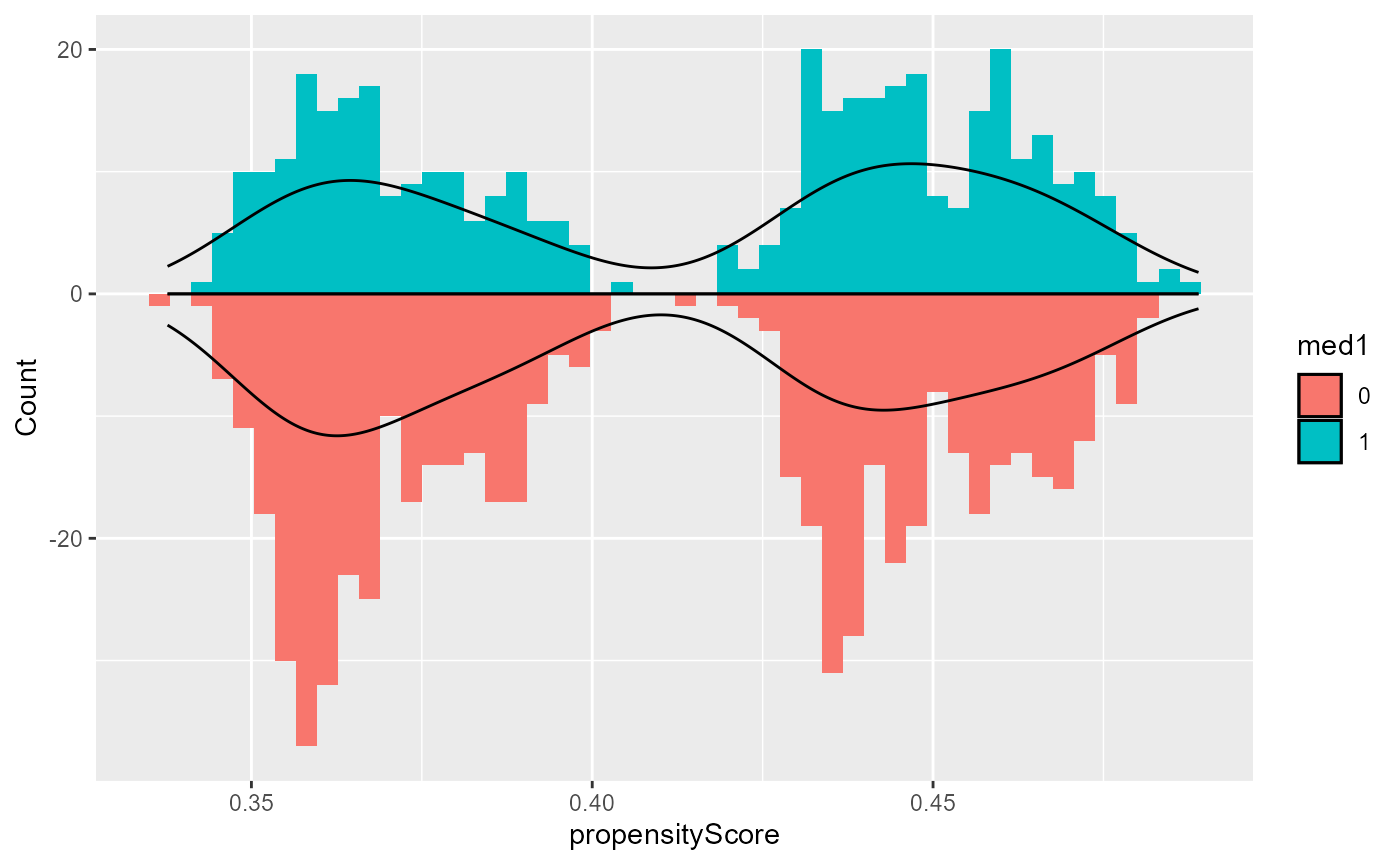
base::plot(result, type = "participationHist")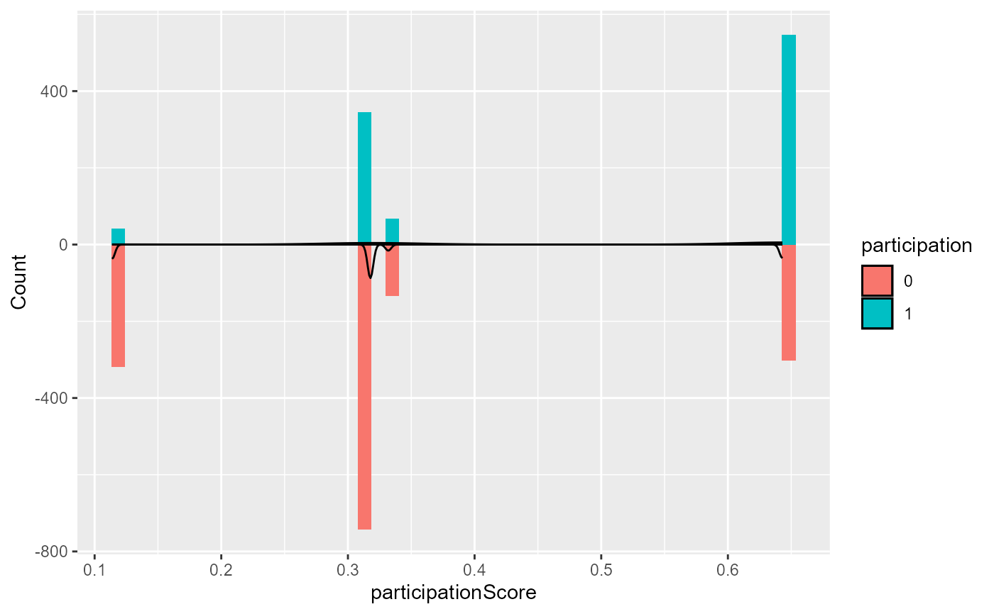
Conditional exchangeability is roughly the assumption
that the only possible confounding is due to the controlled covariates
and effect modifiers. Under this assumption, IOPW estimates will be
reliable if the weighted distributions of covariates and effect
modifiers are similar between treatment groups, and between the study
and target data. This can be (partially) evaluated using standardized
mean differences (SMDs), which are shown in table form by the
summary function. The plot function with
type = "propensitySMD" or
type = "participationSMD" provides graphical versions of
these tables. A general guideline is that an SMD of below 0.1 indicates
balance, but this threshold is arbitrary and left to the choice of the
analyst (Wizard, n.d.a).
base::plot(result, type = "propensitySMD")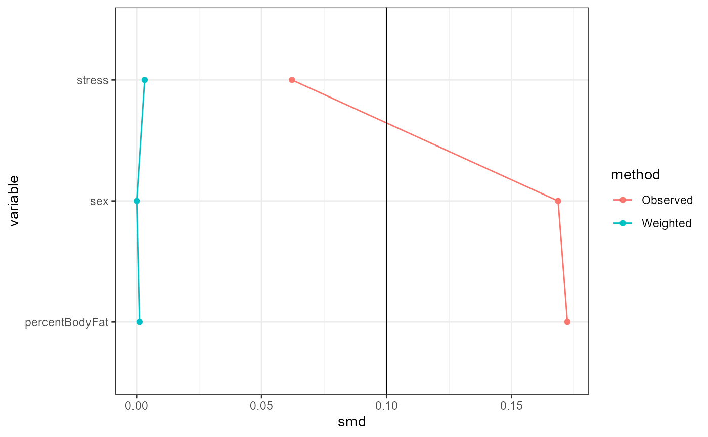
base::plot(result, type = "participationSMD")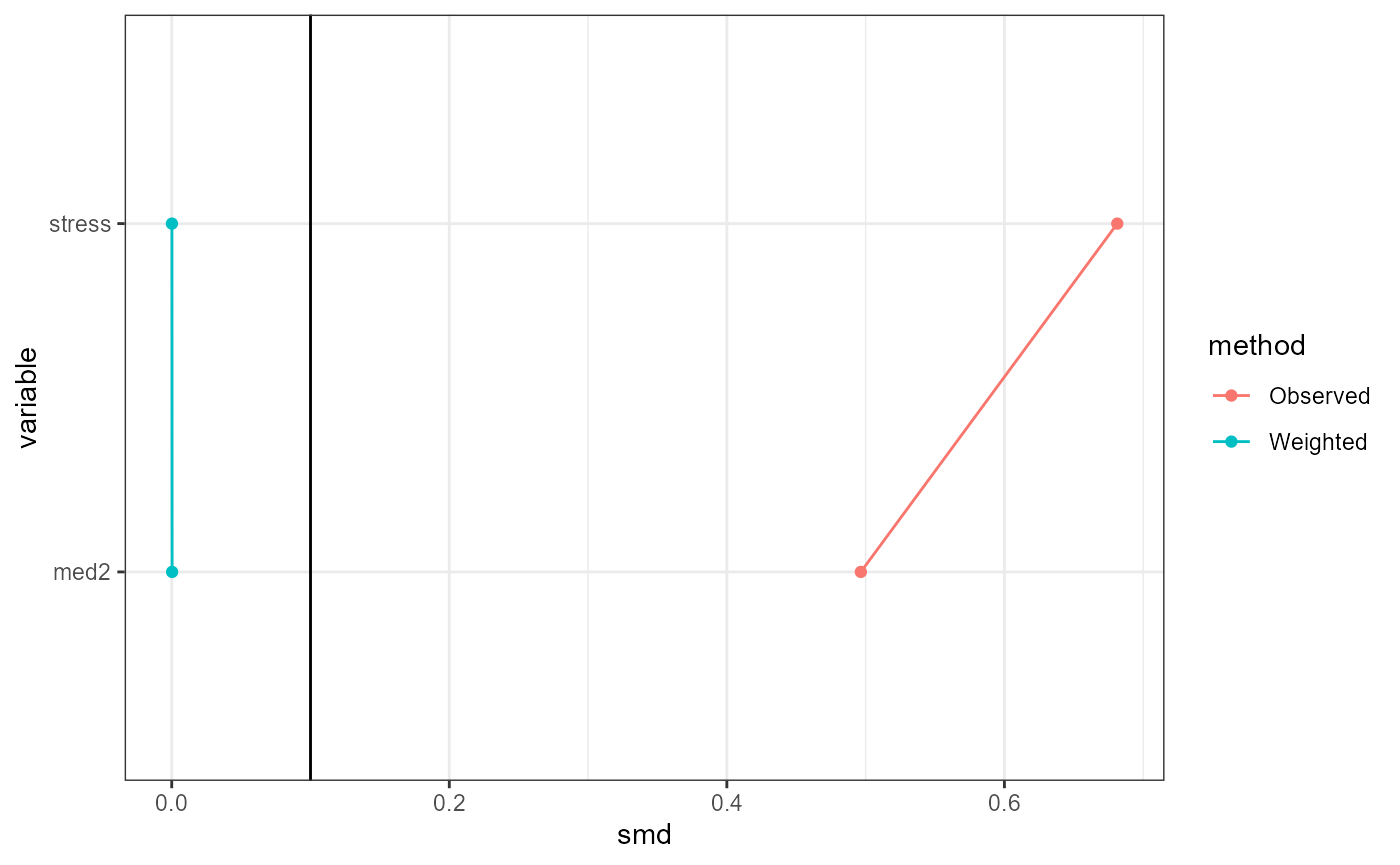
Model coefficient plots showing confidence intervals of the effect
estimates are provided by plot function with
type = "msm". The standard errors are the correct ones
calculated by bootstrap.
base::plot(result, type = "msm")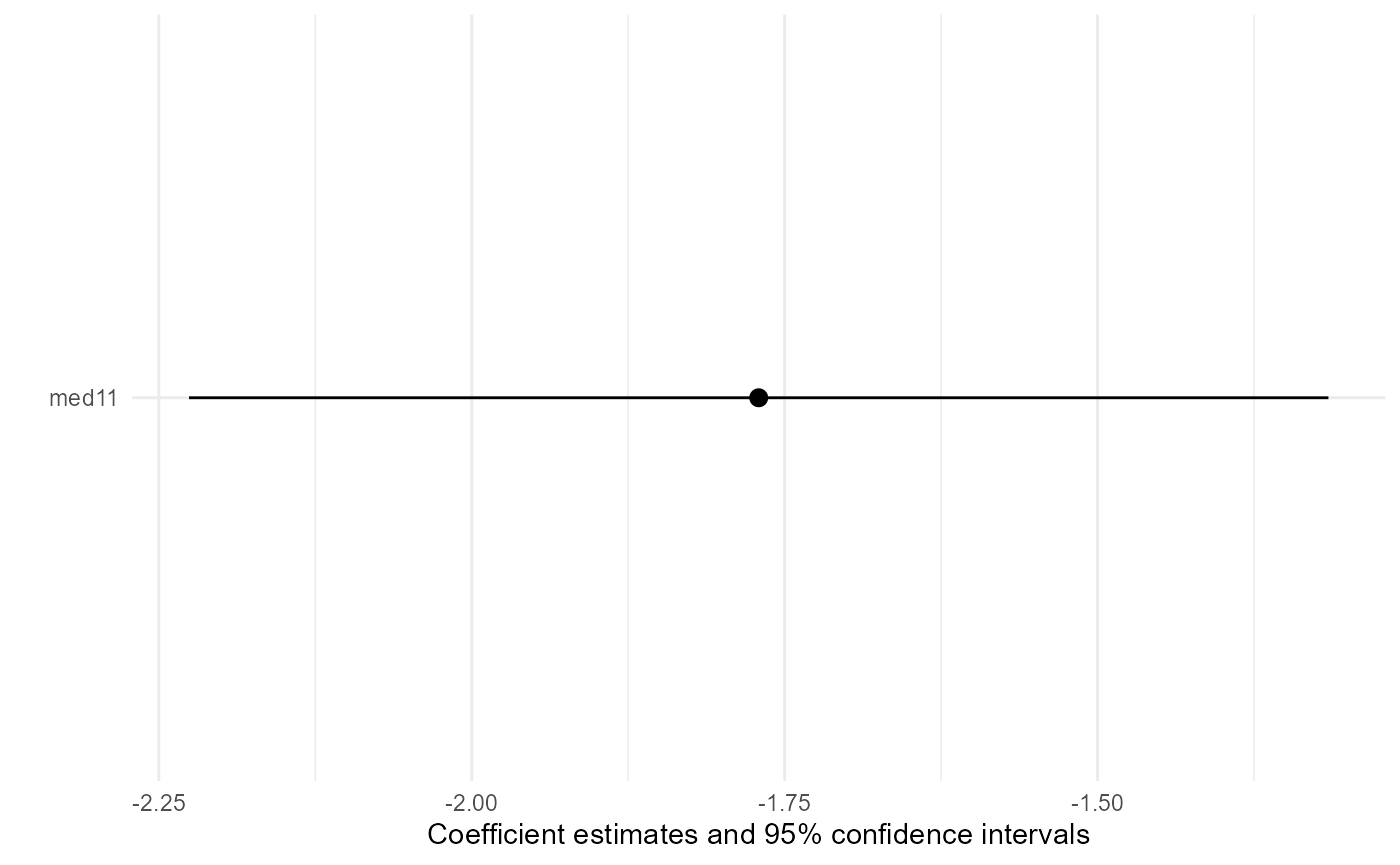
Note that as all plot outputs are designed to be generated with
ggplot2, they can be customized further.